Relational Data
Adithi R. Upadhya
4 August, 2022
Recap
tidyverse package functions like select, group_by, summarize, mutate, filter, case_when, ggplot etc.
Prerequsities
Shortcut of the day
Alt + Shift + K
Shows all keyboard shortcuts!
Relational Data
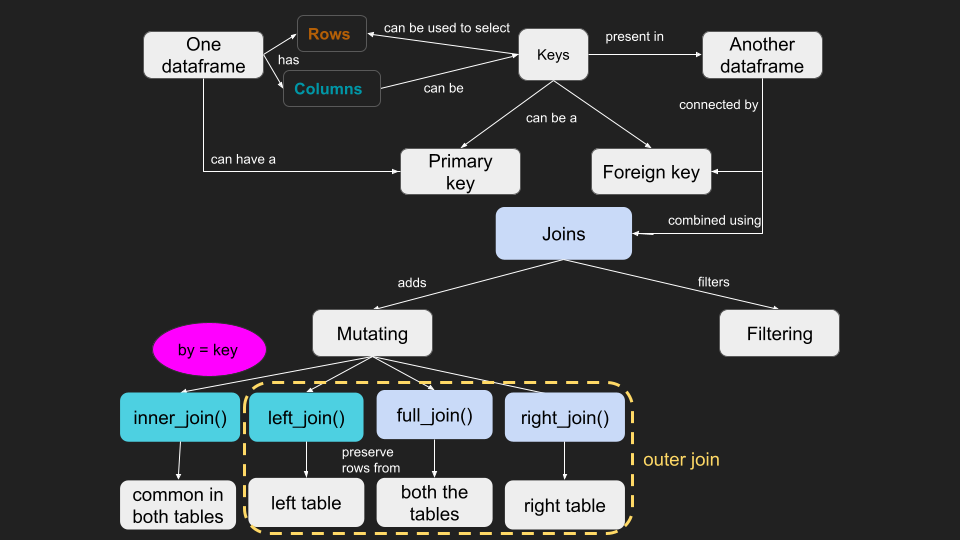
- Usually data is more than one table of data.
- Collectively, multiple tables of data are called relational data because it is the relations that is important.
- Relations are always defined between a pair of tables.
Relationships
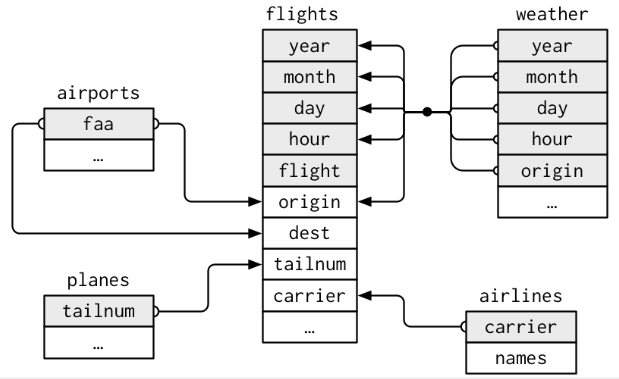
Verbs
Mutating joins, which add new variables to one data frame from matching observations in another.
Filtering joins, which filter observations from one data frame based on whether or not they match an observation in the other table.
Set operations, which treat observations as if they were set elements.
Keys
- The variables used to connect each pair of tables are called keys.
- A key is a variable (or set of variables) that uniquely identifies an observation.
Type of keys
- A
primary keyuniquely identifies an observation in its own table. - A
foreign keyuniquely identifies an observation in another table.
Understanding Keys
- These keys cannot have duplicates. They can be combination of keys as well.
- Sometimes a table doesn’t have an explicit primary key, there a new row can be created as
surrogate keyusingmutate()orrow_number().
A variable can be both a primary key and a foreign key.
Relations
- A primary key and the corresponding foreign key in another table form a relation.
- Relations are typically one-to-many. For example, each flight has one plane, but each plane has many flights.
- many-to-many relations are possible as well. Eg- each airline flies to many airports; each airport hosts many airlines.
Data used
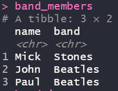
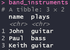
band_members and band_instruments
These data sets describe band members and instruments used by the Beatles and Rolling Stones.
Quiz 1
Imagine you wanted to find out which musician from a particular band played which instrument. What variables would you need? Identify the primary key to be used.
- name, plays; primary key - name
- name, band, plays; primary key - name, band, plays
- name, band, plays; primary key - name
- band, plays; primary key - band, plays
Concept Map

Mutating Join
- A mutating join allows you to combine variables from two tables.
- It first matches observations by their keys, then copies across variables from one table to the other.
Understanding Joins
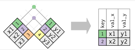
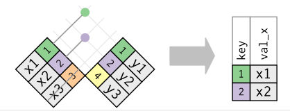
- The colored column represents the
keyvariable: these are used to match the rows between the tables. - The grey column represents the
valuecolumn that is carried along for the ride. - A join is a way of connecting each row in x to zero, one, or more rows in y.
- The number of dots = the number of matches = the number of rows in the output.
Inner Join
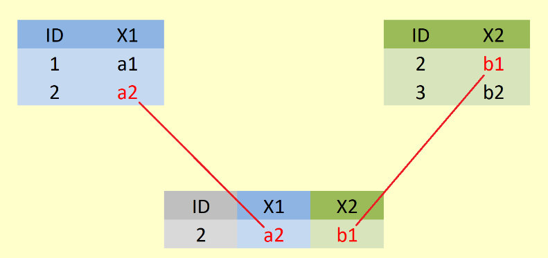
An inner join matches pairs of observations whenever their keys are equal.
The output of an inner join is a new data frame that contains the key, the x values, and the y values.
Demo
Left Join
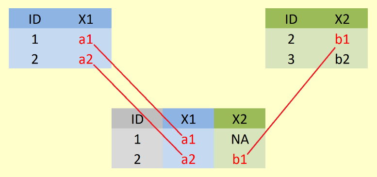
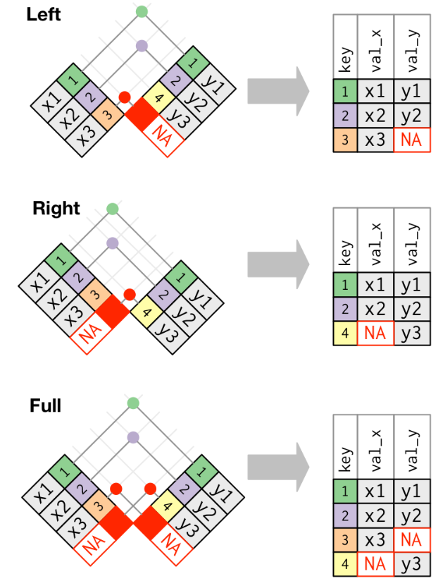
A left join keeps all observations in x.
Demo
Right Join
A right join keeps all observations in y.

Demo
Full Join
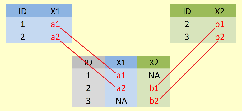
A full join keeps all observations in x and y.
Demo
Outer Joins
Quiz 2
How to combine all observations from the two tables band_members and band_instruments to get a table as shown here.
- left_join
- full_join
- right_join
- inner_join


Defining key columns
- The default,
by = NULL, uses all variables that appear in both tables, the so called natural join. - A character vector,
by = "x". This is like a natural join, but uses only some of the common variables. - A named character vector:
by = c("a" = "b"). This will match variable a in tablexto variablebin tabley.
Concept Map
Filtering Joins
Affect the observations, not the variables. Never have duplicate rows.
semi_join(x, y)keeps all observations inxthat have a match iny.anti_join(x, y)drops all observations inxthat have a match iny.Anti-joins are useful for diagnosing join mismatches.
Semi join and Anti join

Join Problems
Start by identifying the variables that form the primary key in each table.
Do not empirically look for a combination of variables that give a unique identifier.
Check that none of the variables in the primary key are missing.
Check that your foreign keys match primary keys in another table.
Set Operations
- The final type of two-table verb are the set operations.
- These expect the x and y inputs to have the same variables, and treat the observations like sets.
Set Operations types
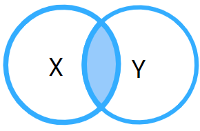
intersect(x, y): return only observations in bothxandyunion(x, y): return unique observations inxandysetdiff(x, y): return observations inx, but not iny
intersect and union

Demo
Quiz 3
How are joins and set operations different from each other? (Choose one or many)
- set operations need same column / variable names while joins do not
- no difference both are same, but have different syntax
- set operations have no keys but joins have keys
Resources
- R for Data Science Chapter 13
- Slides made using Quarto
- Art work by Allison Horst
- For more information on joins